
What Makes a Kernel Fast#
Overview
The roofline model gives a kernel a performance ceiling from memory bandwidth and compute throughput, while arithmetic intensity decides which ceiling applies.
Low arithmetic intensity usually means memory-bound: performance is mainly limited by memory bandwidth. The optimization focus is to reduce HBM traffic, improve reuse, fuse operations, and get as close as possible to the memory-bandwidth roof.
High arithmetic intensity usually means compute-bound: performance is mainly limited by compute throughput. The optimization focus is to keep Tensor Cores busy and reduce idle time on the compute path through overlap.
A kernel is only fast relative to a ceiling. A number like 330 TFLOP/s may look large by itself, but it means something very different on a GPU that can sustain on the order of 2 PFLOP/s on dense fp16 or bf16 Tensor Core work. Without a ceiling, it is hard to tell whether a kernel is close to the hardware limit or still leaving most of the chip idle.
This chapter uses the roofline model to build that reference point, using NVIDIA B200 as the concrete hardware platform. Following the convention from GPU Execution Model, we use rounded ceilings for reasoning: roughly 2 PFLOP/s of dense fp16 or bf16 Tensor Core throughput, and roughly 8 TB/s of HBM3e bandwidth. The exact values depend on the specific device configuration, clock, power limit, and measurement setup. The numbers here should therefore be read as convenient approximate limits for analysis, not exact datasheet constants.
The Roofline Model#
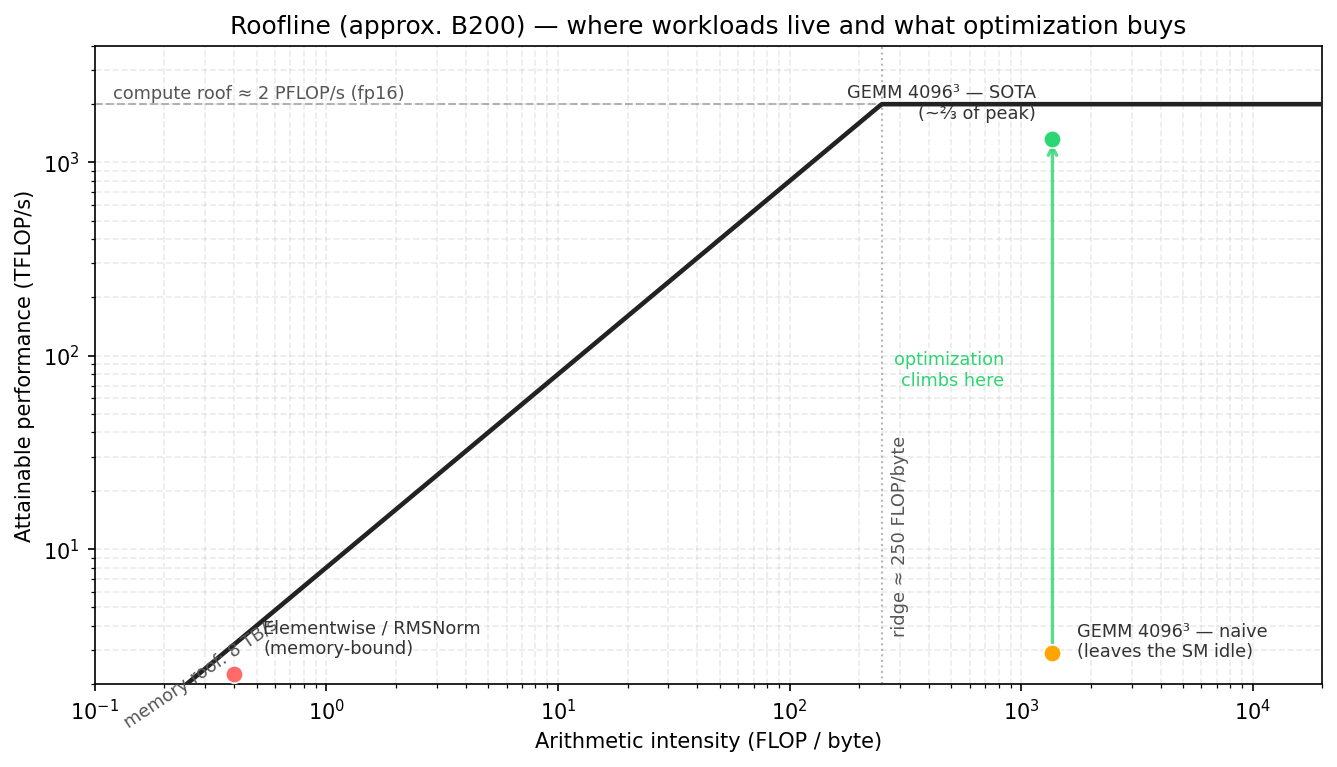
From a performance-analysis perspective, a kernel spends its time on two main activities: moving data and doing arithmetic. The roofline model gives a simple way to reason about this: the kernel’s performance ceiling is jointly determined by the compute-throughput ceiling and the memory-bandwidth ceiling, and more specifically by the lower of the two.
The compute ceiling, or peak compute throughput, is the maximum FLOP/s the hardware can provide on the compute path used by the current kernel. For dense FP16/BF16 Tensor Core GEMM on B200, this ceiling usually comes from Tensor Core throughput. For scalar or elementwise kernels, it may instead come from CUDA cores, special-function units, or some other execution unit.
The memory-bandwidth ceiling can be estimated by multiplying HBM bandwidth by arithmetic intensity. If a kernel does little computation for each byte moved, its performance is usually limited by HBM bandwidth. If each byte supports many operations, the kernel has a better chance of entering the compute-bound region, where the ceiling is more likely to be set by compute throughput.
In units of FLOP/s, the basic roofline bound is:
Arithmetic intensity is:
Here, compute work means the mathematical work the algorithm is actually trying to perform, usually measured in FLOPs, not the total number of instructions executed by the kernel. FLOPs follow the usual convention: one floating-point add or multiply counts as 1 FLOP, and one fused multiply-add, a * b + c, counts as 2 FLOPs. Therefore, for GEMM C = A @ B, if A has shape M × K and B has shape K × N, the GEMM compute work is usually written as:
The memory level must be specified. For an HBM roofline, the bytes are HBM bytes. For an L2 roofline, they are L2 bytes. For an SMEM roofline, they are shared memory bytes. In this chapter, the default roofline is the HBM roofline.
On a roofline plot, the x axis is arithmetic intensity, measured in FLOP/byte. The y axis is the performance the kernel can reach. The memory-bandwidth ceiling is a sloped line:
The compute-throughput ceiling is a horizontal line:
The point where this horizontal line intersects the memory-bandwidth line is called the ridge point, the boundary between memory-bound and compute-bound behavior:
Using the B200 round numbers from this chapter, the ridge point has units of FLOP/byte:
A kernel therefore needs to produce roughly 250 FLOPs for every byte it moves from HBM before it can escape the HBM bandwidth limit and approach the Tensor Core compute-throughput ceiling in this rough model. In other words, under the HBM roofline, a kernel below this arithmetic intensity is memory-bound. It cannot reach peak Tensor Core throughput because it cannot deliver enough bytes per second to keep the compute units fed.
The useful part of the roofline model is not the plot itself. The useful part is that it tells us which resource is limiting performance. A memory-bound kernel does not become fast because its math instructions are slightly better. A compute-bound kernel does not become fast because it saves a few irrelevant bytes. The first step is to know which side of the ridge the kernel is on.
Arithmetic Intensity of Common Workloads#
Arithmetic intensity is often an algorithm property before it is an implementation detail. A rough estimate can usually be made before writing the kernel.
Elementwise and Reductions#
Elementwise kernels, such as GELU, and reduction-style kernels, such as RMSNorm, usually read and write large tensors while doing only a small amount of computation per element.
These kernels therefore tend to have low arithmetic intensity and sit far to the left of the ridge point on the roofline plot. The optimization focus is usually not to add more math instructions, but to reduce HBM traffic and get as close as possible to the memory-bandwidth roof. Common techniques include fusion, which avoids writing intermediate results back to HBM; coalesced or vectorized memory access, which makes neighboring threads or individual instructions access contiguous data more regularly; hardware data movement such as TMA when it applies; and smaller storage dtypes. If there is no data reuse and no fusion opportunity, the memory roof is the true performance ceiling for this class of kernel.
GEMM#
GEMM is the opposite case. Its arithmetic intensity grows with problem size because each loaded tile can be reused for many multiply-accumulate operations.
For a square fp16 matmul with M = N = K, the ideal arithmetic intensity (AI) is approximately:
The unit is FLOP/byte. This estimate assumes A and B are each read once from HBM, C is written once, beta is zero, meaning the old C does not need to be read from HBM and accumulated, on-chip reuse is perfect, and there is no extra metadata, padding, or redundant traffic. Here, metadata means auxiliary information used together with the data, such as the scale in low-precision formats. Real kernels usually move more data than this ideal model, but the estimate is still useful.
Attention#
Attention sits between these extremes. Its arithmetic intensity depends on sequence length, head dimension, tiling, masking, and whether intermediate tensors are materialized.
The key issue in standard attention is the attention-score matrix produced by QK^T. If the kernel writes that score matrix to HBM and later reads it back, it moves a large intermediate through memory. Flash Attention, including Flash Attention 4, raises arithmetic intensity by keeping the relevant tiles on chip and avoiding that HBM round trip.
Attention optimization is therefore partly a roofline problem and partly a scheduling problem. The algorithm is changed so that fewer bytes go to HBM. Then the kernel is scheduled so that the remaining movement and compute overlap.
When Arithmetic Intensity Is Low#
Under the roofline model, if a kernel sits to the left of the ridge point, it is usually considered memory-bound. Performance is mainly limited by HBM bandwidth rather than arithmetic-instruction throughput; Tensor Cores or CUDA cores may sit idle while waiting for data. In this situation, the first question is whether arithmetic intensity can be raised, meaning whether each byte brought from HBM can support more computation.
Fusion is often the most direct method. A common source of low arithmetic intensity is that one kernel writes an intermediate tensor to HBM, and the next operation immediately reads it back. After fusing the producer, which creates the intermediate, with the consumer, which uses it, the intermediate can stay in registers or on-chip storage such as SMEM or TMEM, avoiding that HBM round trip.
Examples include:
GEMM plus elementwise epilogue
normalization fused into a neighboring operator
attention computed without materializing the full score matrix
Another method is blocking for reuse. Blocking means cutting a large problem into smaller tiles, loading each tile into on-chip storage, and reusing it multiple times before eviction. In GEMM, an element of A participates in the computation of many C elements along the same row, and an element of B participates in many C elements along the same column. If each use rereads the value from HBM, HBM traffic becomes large. Compared with an implementation that does not reuse A/B data effectively, blocking keeps A/B tiles on chip so that the same 2MNK mathematical operations correspond to fewer HBM bytes, raising arithmetic intensity under the HBM roofline. Other workloads can use the same idea whenever they repeatedly use the same tile.
We can capture this reuse with a simplified model. For one CTA tile, suppose it computes a B_M × B_N C tile. Each K-stage loads a B_M × B_K A tile and a B_K × B_N B tile, and each element has size s bytes. Looking only at the A/B global memory traffic for this stage, and ignoring C read/write, the arithmetic intensity is approximately:
If B_M = B_N = B, this becomes:
For a concrete example, keep the overall GEMM dimensions M, N, and K unchanged; the total computation 2MNK also stays unchanged. We are only comparing how different CTA tile sizes change on-chip reuse for the same GEMM. Suppose the dtype is FP16/BF16, so s = 2 bytes, and each K-stage uses B_K = 64. If the CTA tile is 16 × 16, this stage performs:
FLOPs. The A/B data read from global memory is:
bytes. The arithmetic intensity with respect to A/B global-memory traffic for this stage is therefore 32768 / 4096 = 8 FLOP/byte. If the CTA tile becomes 64 × 64 while B_K = 64 stays the same, the computation becomes:
and the A/B data read becomes:
bytes. The arithmetic intensity becomes 524288 / 16384 = 32 FLOP/byte. This is the basic roofline intuition behind blocking: as the tile grows, each A/B element read from global memory is reused more times on chip, so the arithmetic intensity with respect to A/B global-memory traffic increases.
Real kernels must also account for C read/write, L2 reuse, occupancy, register pressure, SMEM bandwidth, Tensor Core issue rate, and other factors, so this is only a first-order model. But it captures the core reason blocking raises arithmetic intensity: the same A/B element read from global memory serves more multiply-accumulate operations inside the tile.
Besides increasing on-chip reuse and reducing repeated HBM reads, we can also reduce the number of bytes per value. Moving from fp32 to fp16, fp8, or fp4 reduces data movement and increases the useful computation per byte. However, if these formats require extra metadata, scale factors, or conversion work, the real gain will be smaller than what we would estimate from dtype size alone. A scale factor is the scaling value associated with low-precision data; block-scaled fp8 and fp4 are examples. Even so, smaller dtypes are often one of the most direct ways to move a kernel rightward on the roofline.
If arithmetic intensity is hard to raise further, we have to accept that the kernel is fundamentally memory-bound and change the target to getting as close as possible to the memory-bandwidth roof. A pure copy, a simple elementwise operation, or a single-pass reduction over a large tensor usually does not have enough intermediate data to fuse or enough reuse to exploit. In this case, the optimization focus becomes moving fewer bytes, accessing memory in regular patterns, and keeping the memory pipeline busy:
move each byte once
avoid redundant reads
use coalesced or vectorized accesses
use TMA for regular bulk tiles
keep enough memory requests in flight so the memory pipeline does not sit idle
Once a memory-bound kernel reaches the memory roof, further compute optimization does not help. The only way to go faster is to change the algorithm so it moves fewer bytes.
The Optimization Ladder#
The roofline model can help us identify a kernel’s performance ceiling, but it does not say how much implementation work is needed to approach that ceiling.
A large fp16 GEMM may be compute-bound in theory. That only means the HBM-level memory roof is not the main limit; it does not mean any implementation will reach the Tensor Core compute roof. Closing the gap requires the right instructions, layouts, staging, synchronization, and scheduling. The later GEMM chapters show this on B200 through a sequence of steps: each step keeps the same basic algorithm but changes how the tile is computed or scheduled.
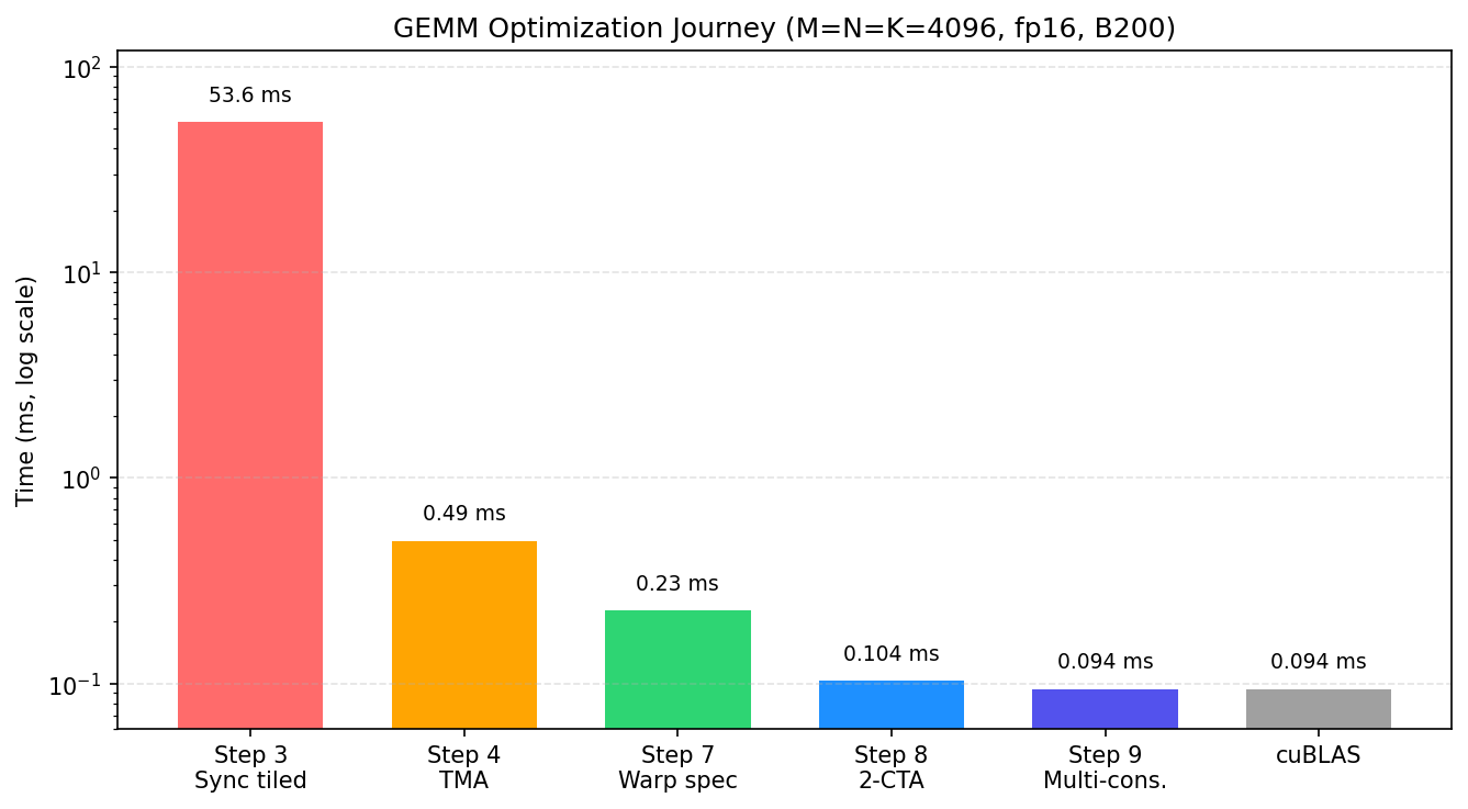
In the GEMM optimization ladder, the first large measured jump is the move from the thread-copy tiled path to the TMA-backed path. The former uses ordinary CTA threads to copy tiles from GMEM to SMEM; the latter delegates this regular tile movement to the TMA hardware engine, letting the kernel feed Tensor Cores through hardware-managed bulk copies.
After that first jump, the main improvements come from overlap and scheduling. TMA brings future tiles into shared memory. tcgen05.mma runs matrix multiply asynchronously. The epilogue handles the output side for results that have already been computed, for example reading out accumulators, performing necessary conversions, and writing back to memory. Software pipelining and warp specialization arrange these pieces so multiple hardware engines can remain active at the same time.
Some intermediate steps do not necessarily speed things up immediately. A step such as warp specialization may temporarily spend resources on a new structure, and that structure may not immediately improve the measured number. It can still be the right step if it enables later, more complex overlap that the simpler structure could not express.
The figure below gives the optimization route developed in the later GEMM chapters. For now, treat it as a roadmap: each point corresponds to an implementation structure, and later chapters explain what TMA, warp specialization, CTA clusters, and multi-consumer execution each change.
Overlap Is the Main Lever#
Once a GEMM is compute-bound and already uses Tensor Cores, the remaining gap usually comes from hardware idle time.
A simple kernel might do this:
load tile k
compute tile k
store tile k
load tile k + 1
compute tile k + 1
store tile k + 1
That schedule leaves hardware idle. While the load runs, the Tensor Core waits. While the Tensor Core runs, the copy engine may be idle. While the store drains, both may be waiting.
A pipelined kernel instead tries to run independent stages together:
load tile k + 1
compute tile k
store tile k - 1
This is the central idea behind the Blackwell kernel structure used later in the book. TMA handles asynchronous data movement. tcgen05.mma handles asynchronous Tensor Core work. The epilogue and stores handle output-side processing and writeback. mbarrier objects connect the stages so that each consumer waits only when the data it needs is actually required.
The point is not to remove dependencies. The point is to schedule around them. The MMA for tile k cannot start until tile k is loaded. The epilogue for tile k cannot read the accumulator until the MMA for tile k is complete. But the load for tile k + 1 can often run while the MMA for tile k is in flight, and the store for tile k - 1 can often drain at the same time.
This is why so many later chapters focus on asynchronous mechanisms:
TMA: global memory to shared memory movement
mbarriers: load completion and resource handoff
tcgen05: asynchronous Tensor Core compute
TMEM: long-lived accumulator storage
warp specialization: separation of producer and consumer roles
clusters: larger cooperative tiles and multicast
They are different mechanisms, but they serve the same scheduling goal: keep useful work running on more than one hardware path at once.
Occupancy and Resource Pressure#
Besides overlap, GPUs can also hide latency by increasing SM occupancy.
SM occupancy describes how much work is resident on one SM at the same time. If one warp stalls because it is waiting on data or a dependency, the scheduler can switch to another warp that is ready. This hides latency by keeping a pool of independent, ready-to-schedule warps available.
SM occupancy is limited by the resources available on each SM. The main limits are registers, shared memory, warp slots, and CTA slots. Warp slots and CTA slots can be understood as the maximum number of warps and CTAs an SM can hold at once. If a kernel uses many registers per thread or a large amount of shared memory per CTA, fewer CTAs or warps can fit on the SM, leading to lower occupancy.
Many modern Tensor Core kernels intentionally spend resources in ways that reduce occupancy. Multi-stage shared memory pipelines consume SMEM. Large register fragments consume registers. TMEM allocations consume Tensor Memory capacity. Warp specialization may reserve whole warps for producer or consumer roles.
This is a deliberate tradeoff. Instead of hiding latency by keeping many unrelated warps resident, these kernels hide latency through explicit overlap inside a smaller number of resident CTAs. A low-occupancy kernel can still be fast if its pipeline keeps TMA, Tensor Cores, and the store path doing useful work.
Neither approach is universally better. Some kernels need high occupancy because they have irregular memory access or limited explicit overlap. Others need deeper staging and specialization, meaning more complex data staging and role separation, because that is the only way to keep driving the Tensor Cores. The right question is not whether occupancy is high, but whether the key hardware units are being used continuously and effectively.
What This Means for Later Chapters#
The later chapters in this book keep returning to the same diagnostic framework:
Which roof is this kernel under?
What resource is binding?
What change moves the kernel closer to that roof?
For memory-bound kernels, the optimization focus is usually not to add more computation, but to reduce unnecessary data movement and make the actual memory accesses get as close as possible to the hardware bandwidth peak. Reducing repeated reads and writes, improving coalescing, improving data layout, or fusing multiple operations all serve to reduce bandwidth pressure.
For compute-bound kernels, with large GEMM as the typical example, the core question becomes how to keep the compute units busy. The first step is of course to use Tensor Cores, but using Tensor Cores is not enough. The kernel also has to stage operands into appropriate on-chip storage ahead of time, form a pipeline with asynchronous data movement and asynchronous MMA, and overlap load, compute, and store as much as possible instead of making Tensor Cores wait for data.
Flash Attention sits between these two styles. It first raises arithmetic intensity by keeping score tiles and probability tiles on chip, avoiding the need to write the full attention matrix back to HBM. After that, it uses the same optimization tools as high-performance GEMM: tiled data movement, shared memory staging, asynchronous compute, and precise resource handoff between execution stages.
In practice, we can optimize a kernel by following this sequence: estimate arithmetic intensity, find the corresponding performance ceiling, decide whether the kernel is closer to memory-bound or compute-bound, and then optimize the resource that actually limits performance.
Without this diagnosis, kernel optimization easily becomes parameter tuning by feel. With it, every change has a clear purpose: it either raises arithmetic intensity, moves the memory path closer to the bandwidth peak, or reduces idle time on the compute units.